Revisit Linear Inverse Reinforcement Learning

“What I cannot create, I do not understand” – Richard Feynman

This is a summary of Ng & Russell’s paper: Algorithms for Inverse Reinforcement Learning . In the spirit of understanding the algorithm inside-out, I implemented my own one with Python. Code is available at github

Notations

MDP is a tuple $(S, A, \{P_{sa}\}, \gamma, R)$

• $S$ is a finite set of $N$ states.
• $A = \{a_1, .., a_k\}$ is a set of $k$ actions.
• $P_{sa}(s')$ is the state transition probability of landing at state $s'$: $P(s, a, s')$ upon taking the action $a$ at state $s$.
• $\gamma \in [0, 1)$ is the discount factor.
• $R: S \rightarrow \mathbf{R}$ is the reward function bounded by value $R_{max}$.

Assumptions

• Expert always performs optimal actions and achieves higher expected value on each state.
• The dynamics of the MDP is known ($\{P_{sa}\}$ is known).

Note that the second assumption is very strong. In most of the real-world problems, we do not get access to the environment’s dynamics.

Algorithm 1

Let’s first go through the algorithm step by step and finally formulate the problem as a linear programming problem.

From the Bellman equation,

$$V^{\pi}(s) = R(s) + \gamma \sum_{s'} P_{s\pi(s)} (s') V^\pi(s')$$

We have:

$$\mathbf{V^\pi} = \mathbf{R} + \gamma \mathbf{P}_{a^*} \mathbf{V^\pi} \\ \mathbf{V^\pi} = (\mathbf{I} - \gamma \mathbf{P}_{a^*})^{-1} \mathbf{R}$$

Note that there $\mathbf{P}_{a^*}$ is a $N\times N$ matrix, $\mathbf{V^\pi}$ and $\mathbf{R}$ are $N\times 1$ vectors.

From the first assumption (Expert always achieves higher expected value on each state) above,

$$\mathbf{P}_{a^*} \mathbf{V^\pi} \succeq \mathbf{P}_{a} \mathbf{V^\pi}, \forall a \in A \setminus a^{*} \\ \mathbf{P}_{a^*} (\mathbf{I} - \gamma \mathbf{P}_{a^*})^{-1} \mathbf{R} \succeq \mathbf{P}_{a} (\mathbf{I} - \gamma \mathbf{P}_{a^*})^{-1} \mathbf{R} , \forall a \in A \setminus a^{*} \\ (\mathbf{P}_{a^*} - \mathbf{P}_{a}) (\mathbf{I} - \gamma \mathbf{P}_{a^*})^{-1} \mathbf{R} \succeq 0, \forall a \in A \setminus a^{*}$$

The last inequality above forms our main constraints for the LP. Note that $(\mathbf{P}_{a^*} - \mathbf{P}_{a}) (\mathbf{I} - \gamma \mathbf{P}_{a^*})^{-1} \mathbf{R}$ represents the gap of expected value on each state between acting optimally and acting suboptimally.

Let’s talk a look at the objective then. The key idea in this paper is to find a reward function $R(s)$ such that it maximize the gap between expert policy and any other policies. To do so, on each state, we want to maximize the gap of expected value of acting optimally and the best expected value of taking suboptimal actions. Following this heuristic, the objective is,

$$\text{maximize} \sum_{i=1}^N \text{min}_{a \in A \setminus a^*} \{\mathbf{P}_{a^*}(i) - \mathbf{P}_{a}(i)\} (\mathbf{I} - \gamma \mathbf{P}_{a^*})^{-1} \mathbf{R}$$

The paper also mentioned to add a $l_1$ regularization term $\|R\|_1$ in the objective to add penalty on large abs value of the reward,

$$\text{maximize} \sum_{i=1}^N \text{min}_{a \in A \setminus a^*} \{\mathbf{P}_{a^*}(i) - \mathbf{P}_{a}(i)\} (\mathbf{I} - \gamma \mathbf{P}_{a^*})^{-1} \mathbf{R} - \lambda \|R\|_1$$

The LP formulation

$$\text{maximize} \sum_{i=1}^N \text{min}_{a \in A \setminus a^*} \{\mathbf{P}_{a^*}(i) - \mathbf{P}_{a}(i)\} (\mathbf{I} - \gamma \mathbf{P}_{a^*})^{-1} \mathbf{R} - \lambda \|R\|_1\\ \text{s.t. } (\mathbf{P}_{a^*} - \mathbf{P}_{a}) (\mathbf{I} - \gamma \mathbf{P}_{a^*})^{-1} \mathbf{R} \succeq 0, \forall a \in A \setminus a^{*} \\ |R_i| \leq R_{max}, i = 1,..,N$$

We can introduce dummy variables to get rid of the non-linear $min$ and l1 norm operations in the objective. Details are in the implementation and thus omitted.

Algorithm 2 - Large State Space

When the state space becomes large (i.e. continous space), the above algorithm becomes intractable. The paper proposed reward approximation to address this limitation,

$R(s) = \sum_j \alpha_j \phi_j(s), \text{for }j = 1, .., d$ Where, $\{\phi_j\}$ are features functions (the original paper: “fixed known, bounded basis functions”) mapping from $S$ into $\mathbf{R}$.

Let $V_j^\pi$ denote the value function of the policy $\pi$ when the reward function is $R = \phi_j$, then,

$$V^\pi = \sum_j \alpha_j V_j^\pi$$

From the assumption that the expert acts optimally,

$$\mathbf{E}_{s'\sim P_{sa^*}} [V^\pi(s')] \geq \mathbf{E}_{s'\sim P_{sa}} [V^\pi(s')], \forall a\in A \setminus a^*$$

There are two problems with this formulation:

• Since the state space is large, we could not enumerate all the constraints, therefore, we can only sample $S_0$ from the state space.
• Since we used the linear approximation of the reward, we could not guarantee that the with expressed reward function, the optimal function is still optimal. Thus the above inequalities are not guaranteed to be always hold. To address this, the paper introduced a penalty mechanism to relax the original constraints: penalize larger on the constraints that are not held.

The LP formulation

$$\text{maximize} \sum_{s\in S_0} \text{min}_{a\in A \setminus a^*} \{ p(\mathbf{E}_{s'\sim P_{sa^*}} [V^\pi(s')] - \mathbf{E}_{s'\sim P_{sa}} [V^\pi(s')]) \} \\ \text{s.t. } |a_i| \leq 1, i = 1,..,d$$

Where $p(x) = x$ if $x\geq 0$, $p(x) = 2x$ otherwise.

Implementation & Experiment

The algorithm 1 is implemented. This algorithm requires full access to the transition dynamics of the environment, i.e. $\{P_{sa}\}$. This makes the gridworld a perfect test bed for the algorithms since its dynamics is known.

I experimented the algorithm on a 10x10 stochastic gridworld (with 70% acting according to the action, 30% randomly), $gamma = 0.5$ and $\lambda=10$, the results are in the figures below. The upper right value map was solved by value iteration.

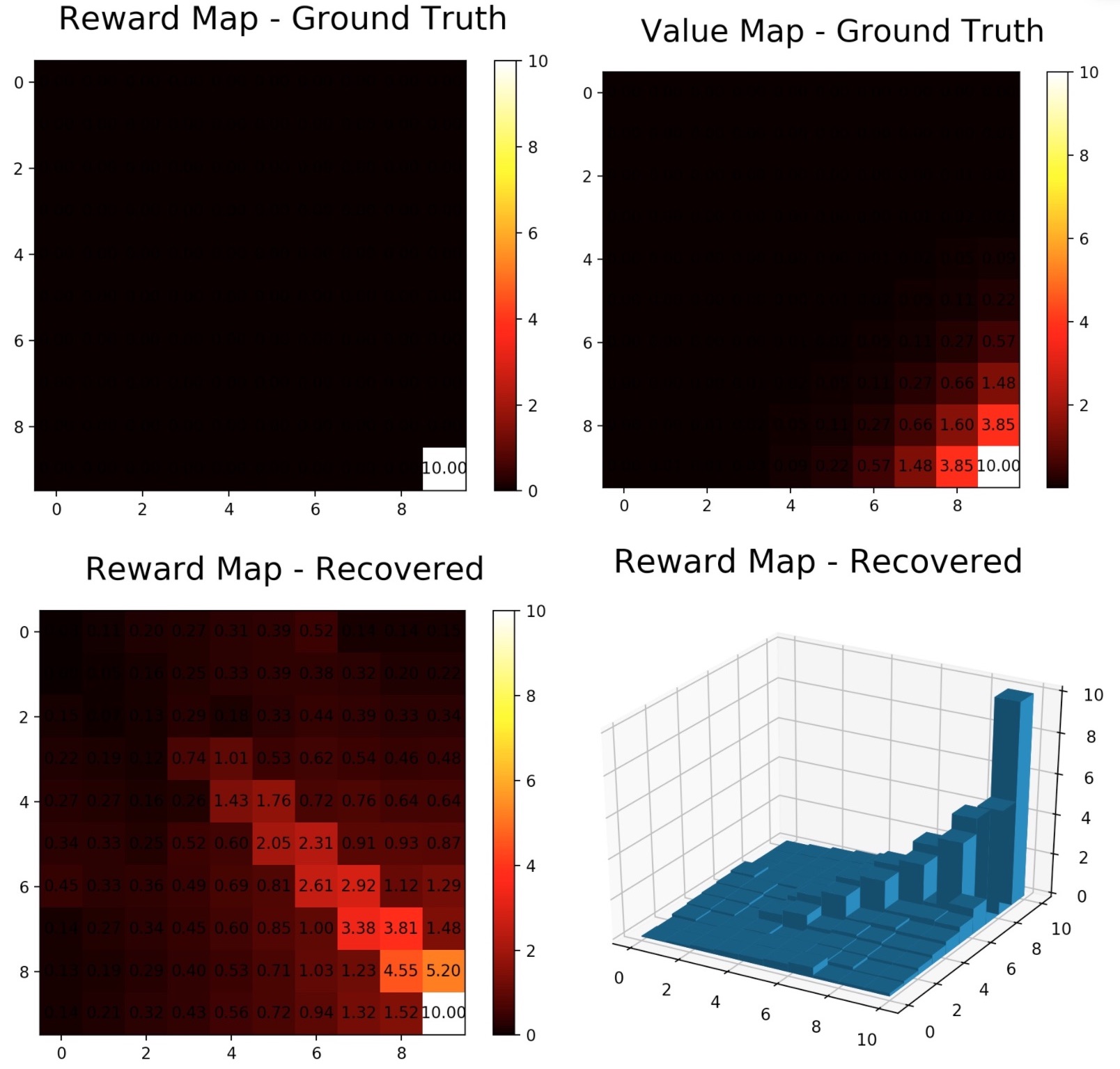
Since implementing this algorithm is solely for educational purposes to catch up with the latest works, I did not do thorough experiments due to time limitation.

Limitations

• Assumes expert’s policy is optimal
• Requires full access to the transition dynamics

In terms of the second limitation, we can use Monte Carlo (MC) to estimate dynamics of the environment. In this case, the limitation becomes requiring access to the environment (mdp) or large enough trajectories.